Lab: clean the sales sheet and answer four questions
A messy export arrives. Make it a clean table, then get four answers out of it that you would be happy to repeat to the owner.
The situation
The owner forwards a sales export: a title row above the headers, a Region column with “North”, “north” and “N”, amounts with a dollar sign typed in, a blank row between months, and a totals row at the bottom. She wants four answers by lunchtime:
- Which region dropped the most from last month to this month?
- What did we take in total for one category?
- How many orders meet a condition (for example, Paid and over 500)?
- Which formula should sit in the summary cell so the answer updates next month?
Clean first, then answer
Answers from a dirty sheet are wrong in ways you cannot see. Work in this order:
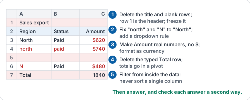
| Step | What to do | Lesson |
|---|---|---|
| 1 | Delete the title row and the blank rows; make row 1 the header; freeze it | 1 |
| 2 | Fix spelling variants in Region and Status (filter to each odd value and correct it); add a dropdown rule | 1, 3 |
| 3 | Make Amount a real number column (values on the right of the cell); format as currency | 1 |
| 4 | Delete the typed totals row; totals belong in a summary block or pivot | 1 |
| 5 | Turn on a filter from a cell inside the data; never sort a single column | 2 |
The export as it arrives, with the five steps mapped onto it.
Getting the four answers
- Biggest drop: pivot with Region in Rows, Month in Columns, SUM of Amount in Values. Subtract this month from last month for each region, or read the two columns side by side. “Dropped the most” means the largest fall in money unless the owner says percent.
- Total for a category:
=SUMIF(category range, "Category", amount range), or read the pivot row. - Count meeting a condition:
=COUNTIFS(status range, "Paid", amount range, ">500"), or filter to the condition and count the rows shown. Watch the boundary: “over 500” excludes exactly 500. - Which formula: state what the owner wants in words (total, count, average, lookup) and match it: SUM, SUMIF, COUNTIF, AVERAGE, XLOOKUP.
Check each answer a second way. A pivot total and a SUMIF should agree; if they do not, there is still a dirty cell.
What the assessment asks
The lab items show you a small seeded table, up to a dozen rows, and ask one of the four questions. Read the headers, work the answer out from the rows shown, and type just the answer: a region name, or a plain number with no currency sign or commas. Take the time you are given; a calm second read of the rows is worth more than speed.
Try it now
Export or copy any real sales or expense list into a new sheet. Do the five cleaning steps, build one pivot, and write one SUMIF and one COUNTIF that agree with the pivot. Note how long it took; next time it will be half that.
Remember: clean first, answer second, check each answer a second way. Then type only what was asked for.
Checking your progress…