Formulas 2: IF and XLOOKUP
IF makes a decision for each row. XLOOKUP fetches a value from another table so nobody retypes prices.
IF: a decision per row
=IF(test, value if true, value if false)
The test compares something and is either true or false. Examples, assuming hours are in E2:
| Formula | E2 is 38 | E2 is 44 |
|---|---|---|
=IF(E2>40, "Overtime", "OK") |
OK | Overtime |
=IF(E2>=40, "Full week", "Part week") |
Part week | Full week |
=IF(E2=0, "Absent", "Present") |
Present | Present |
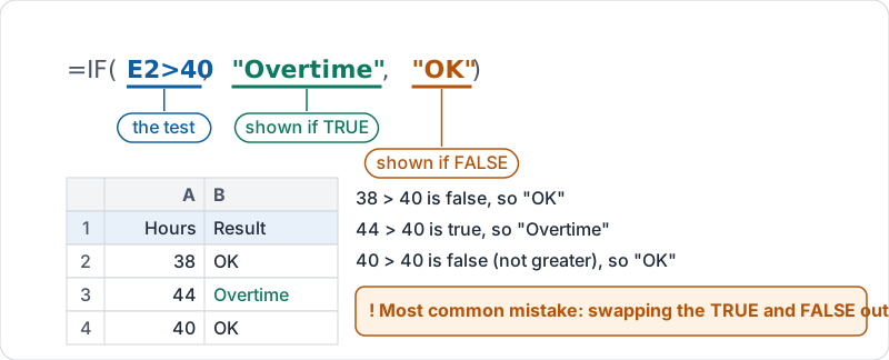
Read the order carefully: the second input is what shows when the test is true. Swapping the two outputs is the most common IF mistake, and the sheet will not warn you.
The three inputs of IF, and three rows run through it.
The outputs can be numbers or other formulas: =IF(C2>1000, C2*0.05, 0) gives a 5 percent commission on big sales and nothing on small ones.
If you find yourself nesting IF inside IF three deep, stop. Use IFS (several tests in a row) or a lookup table with XLOOKUP instead.
XLOOKUP: fetch from another table
Prices, names and rates belong in one place. XLOOKUP pulls them into your working sheet so nothing is retyped.
=XLOOKUP(what to find, where to look, what to return)
Sample price list, SKU in A, Product in B, Price in C, rows 2 to 7:
| Row | A SKU | B Product | C Price |
|---|---|---|---|
| 2 | BK-100 | Brake pads | 48 |
| 3 | BK-200 | Brake rotor | 92 |
| 4 | FL-010 | Oil filter | 14 |
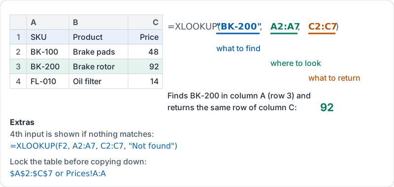
=XLOOKUP("BK-200", A2:A7, C2:C7) returns 92: it finds BK-200 in column A and returns the value from the same row of column C. Point the first input at a cell (=XLOOKUP(F2, A2:A7, C2:C7)) and it looks up whatever SKU is typed in F2.
Two useful extras:
- A fourth input is what to show if nothing matches:
=XLOOKUP(F2, A2:A7, C2:C7, "Not found"). Without it you get an error. - The lookup column can be anywhere, left or right of the result column. That is the main reason XLOOKUP replaced the older VLOOKUP, which could only look to the right.
One lookup, traced through the price list.
Lock a range before you copy
When you copy a formula down a column, its ranges shift down too. For a lookup table that must stay put, lock it with dollar signs: $A$2:$C$7. Or put the table on its own sheet and refer to whole columns: Prices!A:A.
IFERROR for tidy sheets
Wrap any formula that might fail: =IFERROR(XLOOKUP(F2, A2:A7, C2:C7), ""). A blank beats a red error cell in a report, but only when the blank is honest.
Try it now
Make a two-column list of five products and prices on a sheet called Prices. On another sheet, type a product name in A2 and put =XLOOKUP(A2, Prices!A:A, Prices!B:B, "Not found") in B2. Change A2 and watch B2 follow. Then add an IF in C2 that shows “Premium” when B2 is over 100 and “Standard” otherwise.
Remember: IF decides, XLOOKUP fetches. Check the true and false outputs are in the right order, and give XLOOKUP a “not found” value.
Checking your progress…